The New PAMGuard MATLAB Library

PAMGuard 2 came out a few months ago. You might have noticed it doesn’t look or feel very different from PAMGuard 1.1xx (apart form the new display detailed in a previous blog post). So why has the number been bumped up? The main reason is that the PAMGuard team has done an extensive rewrite into how data is handled under the hood. The Binary files in which data are saved are now different and no longer backward-compatible (you can’t open them with previous versions of PAMGuard). The main reason behind this was to give each data unit a unique ID number to make it much easier to find and reference. There was also a large tidy-up and restructuring of all the code dealing with data handling – if you’re a developer it makes it a lot easier… Anyway, we won’t nerd-out too much on that. The upshot of all of this is that the new data units made it possible to write a much nicer MATLAB library for opening data processed in PAMGuard and this post is going to show you how to use it.

PAMGuard and MATLAB.

Why do you even have ‘Binary Files’ and why are the called that? PAMGuard connects to a database and technically you can save everything to the database (File->Storage Options). The problem with this is that for some detectors, e.g. the click detector, you can have thousands of data units in a minute. This is too much for the generic data handling of a database and slows things down a lot. A much faster way to save the data is to simply to convert each data unit into a list of numbers in a known format, and fire that list straight into a file – the Binary File. So Binary files are generally used to save data which can get above a few megabytes, e.g. clicks, whistle/moan contours and noise, but not things like GPS data which are generally only one or two measurements per second.

And why do we call them binary files?– Technically they save data as binary (zeros and ones) but so do all computers files. So the answer to that one is I don’t know.

Why do we have a MATLAB library to read in PAMGuard binary files? The main reason is that PAMGuard can’t do everything. Sometimes, your research questions require you to have more individual control in carrying out specific analyses with your data, and so being able to open that data in a sensible format is important. You can alternatively export a lot of data to the database which can then be opened as a spreadsheet but this can be slow and some parts of data units, e.g. waveforms, can’t be exported to the database at this time.

Why MATLAB? This is a bit of a contentious issue. My personal opinion is that for science, MATLAB is a great language. It’s simple, has an amazing library of functions, and has excellent supporting documents. But it’s a bit slow sometimes and very, very expensive. That goes against the ethos of free open source software so an R, Python, and/or Octave library should also exist (stay tuned).

Where can you get the library? The library is hosted online. You can either download it as a single zip file, or you can use something like Tortoise SVN to check it out to a folder on your computer and keep it up to date as changes and bug fixes are made.

27/03/2020 Update: The amazing folks at NOAA have made an R library for PAMGuard that closely follows the MATLAB function names. Check it out on github. 

Tutorial

The following code is a tutorial on the new PAMGuard MATLAB library. Make sure you’ve downloaded the PAMGuard MATLAB library and that it’s added to your MATLAB path. This was tested on MATLAB 2016/17. Older or new versions might vary a bit.

Data

The data set we’ll use for this example contains dolphin whistles collected by a stereo towed hydrophone array. Here is the .wav file we’ll be using. It’s mostly within human hearing range @48kHz sampling frequency.

.

I used the .psf file bundled in PG_whistles_clicks which also contains the database and binary files which were created during analysis. It’s best to have a go at running the analysis in PAMGuard yourself, but if you don’t have the time or the inclination, then use the Binary files I created for the rest of the tutorial. Remember, to analyse the data, make sure you’re using PAMGuard version 2.0+. You can download it at http://www.pamguard.org

Analysing the data in PAMGuard real time mode. Lots of whistles and lots of clicks.

Using the MATLAB library

Opening a single binary file is really easy. In the first version of the PG MATLAB library you needed to know what file you were opening. So clicks were opened with a function loadClickFile(), whistles were opened with loadWhistleFile(), etc. In the new version, however, you simply input the binary file name into the function loadPamguardBinaryFile(). Here’s an example with a whistle file.

file='C:\WhistlesMoans_Whistle_and_Moan_Detector_Contours_20170116_183344.pgdf';

[pgdata fileInfo]=loadPamguardBinaryFile(file);

This piece of code opens a binary file, which contains some whistles. To open a click file, simply change the file path to a click binary file instead of a whistle binary file.

The pgdata variable is an array of MATLAB structures, each of which represents a single data units e.g. a single whistle detection. The fileInfo variable contains information on the file itself i.e. what version of PAMGuard it was created with, what module the data came from, what the module name was etc. That can be very useful info for datasets that might have been sitting on the shelf gathering dust for a little too long! Note that if you’re not interested in file information you can just load the data units with pgdata =loadPamguardBinaryFile(file). Different types of data unit have different fields within each structure, however they all share a generic set of fields. If you open a single click file and then type:

fieldnames(pgdata(1))

MATLAB will return a list of field names in each structure. Here’s what each of these means…

‘flagBitmap’- a bitmap of flags- these can be used to annotate data units.
‘identifier’ – an extra identifier for the data unit.
‘UID’ – a unique identifier for the data unit. This can be used to easily match data units to super groups or find in large data sets.
‘millis’ – the data/time stamp in milliseconds. This can be converted to MATLAB datenum by using the dateNum2Millis(millis) function.
‘channelMap’ – a bitmap of channels. Shows all channels the detection was made on. This one integer number which can be converted to an array of channels by using the getChannels(channelMap) function
‘startSample’ – the start sample. This relative to the last time the sound card reset.
‘sampleDuration’ – the duration of the data unit in samples.
‘freqLimits’ – the frequency limits of the data unit in Hz. For example this would the high and lowest frequency of a whistle detection. 
‘numTimeDelays’ – the number of time delays within the data unit.
‘timeDelays’ – the time delays between channels in seconds.
‘date’ – the date in MATLAB datenum format.

Click Specific Fields
‘triggerMap’ – the click trigger map.
‘type’ – the click classification flag.
‘flags’ – extra click specific flags.
‘angles’ – angles localisation in radians. The first angle is the heading between -pi and pi or 0 and pi if there is right/left ambiguity.  There be a  second measurement which represents the vertical angle between -90 and 90 degrees.
‘angleErrors’ – errors in angle localization.
‘duration’ – duration in seconds (legacy field).
‘nChan’ – number of channels.
‘wave’ – array of waveforms on each channel. Waveforms are between 1 and -1 which represents the entire dynamic range of the recording DAQ card. Each point is one sample.

Whistle and Moan Specific Fileds

‘amplitude’ – the average amplitude of the whistle contour.
‘sliceData’ – a structure array which contains info on the whistle contour.
‘contour’ – array which represents the whistle contour in the frequency domain. The frequency of each point is contour(i)*samplerate/fftlength.
‘contWidth’ – the width of the contour in units as above.

Some examples

Now we’ll move on to some examples using the library. These are just a few ideas – once you’ve extracted the data, what you can do with it using a programming language is essentially endless.

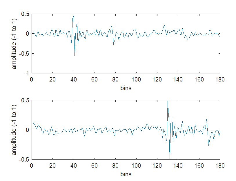
Plotting clicks waveforms

You can easily plot waveforms from individual clicks by simply accessing one of the structures within the structure array, accessing the ‘wave’ field and using MATLAB plot functions. Here’s an example.

 

file = "C:\PAMGuard_whistles_test\Binary\20170116\Click_Detector_Click_Detector_Clicks_20170116_183344.pgdf";

%open the binary file
[clicks, fileInfo] = loadPamguardBinaryFile(file); 

%iterate through all clicks
for i =1:length(clicks)
    %figure out how many waveforms there are
    nwaveforms=clicks(i).nChan;

    %plot each waveform in turn on a single plot.
    for j=1:nwaveforms
        subplot(nwaveforms,1,j)
        plot(clicks(i).wave(:,j));
        ylabel('amplitude (-1 to 1)' )
        xlabel('bins')
        %draw the plot.
        drawnow;
    end

    %move to next click and next plot
end

This might look a bit daunting to those not used to MATLAB, but it’s actually very simple. The first lines open the click file using the PAMGuard MATLAB library. The for i=1:length(clicks) loop then runs through all clicks opened and plots the waveforms. Note how it is very easy to access variable for each data unit. Simply grab the click from the structure array using clicks(i) (where i =1 to the length of the array) and then type what field you’re after e.g. the_date = clicks(7).date.

MATLAB should plot all waveforms from the open binary file. Tip. If you want to control when to move onto each subsequent plot add ‘pause’ inside the outer for loop.

Histogram of clicks amplitudes

The last example wasn’t particularly useful for anything other than learning how the library works. In this next example, we’ll plot the amplitude of all the clicks.

Let’s assume that we used a ±5 V dynamic range soundcard with a pre-amplifier gain of 29 dB and on-board amplifier gain of 60 dB, leading to 89 dB of gain total. Finally, let’s assume the sensitivity of the hydrophones was -201 dB re 1V/μPa. There’s a handy little function called amp = clickAmplitude(clickWave, hSens, gain, adcPeakPeak) which converts from the -1 to 1 amplitude range in PAMGuard Binary files to received dB re 1µPa peak to peak. This is what’s used in the code below to calculate the recieved level of each click.

The first piece of code here is a function (files= findBinaryFiles(folder)) to find all binary files within a folder, including sub folders. The code for the function is below. It’s contained in the legacy binary file folder but this is an improved version so use it instead. I won’t go into too much detail on how it all works to keep the size of this post reasonable but feel free to copy and use.

function [filenames]= findBinaryFiles(folder, containsName)
%FINDBINARYFILES finds all binary file paths within a folder and subfolders
%   [FILENAMES]= FINDBINARYFILES(FOLDER) finds all .pgdf files within a
%   folder and it's sub folders. The function returns a cell array of
%   FILENAMES.
%
%   [FILENAMES]= FINDBINARYFILES(FOLDER, CONTAINSNAME) finds all .pgdf files
%   within a folder that all also contain a string CONTAINSNAME e.g. this
%   could be 'clicks' which would find all click binary files.

if nargin < 2
    containsName=[];
end

filenames={};
subFiles=dir(folder);
for i=1:length(subFiles)

    if (strcmp(subFiles(i).name,'.')==1 || strcmp(subFiles(i).name,'..')==1)
        continue;
    end

    if (subFiles(i).isdir==1)
        subFolderName=[folder,'\', subFiles(i).name];
        filenames=cat(2, filenames,findBinaryFiles(subFolderName,containsName));
    else
        binaryFileName=[folder,'\',subFiles(i).name];
        binaryChar=char(binaryFileName);
        fileEnd=binaryChar(length(binaryChar)-3: length(binaryChar));
        %add to binary file list

        if (strcmp(fileEnd,'pgdf')==1)
            if (isempty(containsName))
                % if no contansName specified then add to list
                filenames=cat(2,filenames ,binaryFileName(1,:));
            elseif (~isempty(strfind(subFiles(i).name, containsName)))
                %if a contansName is specified only add file if it contains
                %the specified string
                filenames=cat(2,filenames ,binaryFileName(1,:));
            end
        end
    end

end
end

The next piece of a code is a script which opens a folder of click binary files, calculates the amplitude and plots a histogram.

%load all click binary files in folder, create one arrya of click
%amplitudes and then plot a histogram.
clear

%the fiolder containing binary files
folder = 'C:\PG_whistles_clicks\Binary\20170116\';

%some info on PAM system
hSens=-201; %hydrophone sensitivity in dB re 1V/uPa
gain=89; %dB
p2pDAQ=10; %the peak to tpeak voltage range of the DAQ system. 

%find the binary files which are for clicks.
clickfiles=findBinaryFiles(folder, 'click');

%create an array of all click amplitude from all binary files. 

amplitudedB=[];
n=1;
%iterate through each file.
for i=1:length(clickfiles)
    % print out something for sanity in case there are lots of files and
    %script takes a very long time.
    disp(['Loading file ' num2str(i) ' of ' num2str(length(clickfiles))])

    %load the file of clicks
    clicks=loadPamguardBinaryFile(clickfiles{i}); 

    %calulate amplitudes for each click
    %pre allocate the array for speed. The array is time and amplitude.
    clickamplitudes=zeros(length(clicks), 2);
    for j=1:length(clicks)
        clickamplitudes(j,1)=clicks(j).date;

        amplitudedB=clickAmplitude(clicks(j).wave, hSens, gain, p2pDAQ);
        clickamplitudes(j,2)=mean(amplitudedB);
    end

    %add to master array
    amplitudedB=[amplitudedB; clickamplitudes];
end

histogram(amplitudedB(:,2),50)
xlabel('amplitude (dB re 1uPa pp)')

All this piece of code does is use <findBinaryFiles(folder, ‘click’) to create a cell array list of binary file paths which contain clicks . It then opens each binary file in turn, calculates the amplitude of all clicks within the file using clickAmplitude(....) and adds to a master click amplitude list (amplitudedB) before going onto the next file and repeating. amplitudedB then contains the amplitudes of all clicks which can be plotted as a histogram using the MATLAB histogram function. Easy right! You should end up with something that looks like

This is what you’d expect to see during a strong encounter. There are two overlapping distributions of clicks. One distribution are the louder dolphin clicks and the other is likely random transient sounds generated from the ship’s propeller and any other noisy acoustic things about. The two distributions mush together to give the bimodal shape above.

whistle contours plotted together

For the last example we’ll plot a bunch of whistle contours on a graph, with each contour starting at time 0.  This lets you view a number of contours overlapping each other which can be useful for visualising data. Really though, it’s just an example of how to plot whistles from the binary files. Here’s the code.

clear
filename='C:\Users\macst\Desktop\PG_whistles_clicks\Binary\20170116\WhistlesMoans_Whistle_and_Moan_Detector_Contours_20170116_183344.pgdf';
tones  = loadPamguardBinaryFile(filename);

samplerate=48000;
fftlength=1024;
hold on;
for i=1:length(tones)
    contour=tones(i).contour*samplerate/fftlength;
    myplot(i)=plot(contour,'g','LineWidth',0.5);

    disp(['Plotting whistle ' num2str(i) ' of ' num2str(length(tones))])
end
hold off
xlabel('slice')
ylabel('frequency (Hz)')

% force MATLAB to draw the graph.
drawnow;

%add transparencty to the whisltes
for i=1:length(myplot)
    myplot(i).Color=uint8(255*[0 1 1 0.1]);
end

This is again not very complicated. In this instance only one of the binary files is opened. The whistles are plotted within a for loop sequentially on the same plot by using the hold on command. Finally the lines on the plot have transparency added to make it easier to see (bit of a hack way of doing it but opacity in MATLAB isn’t well supported). A good challenge would be to expand this code to work with a folder of whistle files and maybe use a nicer colour scheme…

Lots of whsitle contours plotted on top of each other. Is it useful? Probably not, but it’s a good way to learn how to plot detected whistle and moan contours.

The END

I hope this has been a useful brief introduction to the PAMGuard MATLAB library 2.0. It’s a great tool for researchers and there are loads more you can do than just the examples I’ve shown here. Best way to get used to it is to just keep trying things out. Good luck!

Advertisement